Examples of plots
This notebook presents examples of the bff.plot module.
For each function, the ax can be provided and is returned by the
function. This allow to plot multiple things on the same axis and modify
it if needed.
import matplotlib.pyplot as plt
import numpy as np
import pandas as pd

import bff.plot as bplt

np.random.seed(42)
# Variables with fake data to display.
history = {
    'loss': [2.3517270615352457, 2.3737808328178063, 2.342552079627262,
             2.310529179309481, 2.3773420348239305, 2.3290258640020935,
             2.3345777257603015, 2.336566770496081, 2.34276949460782,
             2.321525989465378, 2.3300879552735756, 2.3224288386915197,
             2.324129374183003, 2.3158747431021838, 2.3194296072475873,
             2.2962934024369894, 2.296843618603807, 2.298411148876401,
             2.302087271033819, 2.2869889256942213],
    'acc': [0.085427135, 0.09045226, 0.110552765, 0.110552765, 0.06030151,
            0.14070351, 0.110552765, 0.10552764, 0.09045226, 0.10050251,
            0.11557789, 0.12060302, 0.110552765, 0.10552764, 0.1356784,
            0.15075377, 0.11557789, 0.12060302, 0.10552764, 0.14572865],
    'val_loss': [2.3074077556791077, 2.306745302662272, 2.3061152659403104,
                 2.3056061252970226, 2.30513324273213, 2.3046621198808954,
                 2.304321059871107, 2.304280655512054, 2.3042611346560324,
                 2.3042683235268466, 2.3044002410326705, 2.304716517416279,
                 2.3049982415602894, 2.305085456921962, 2.3051163034046187,
                 2.3052417696192022, 2.3052861982219377, 2.305426104982545,
                 2.305481707112173, 2.3055578968795793],
    'val_acc': [0.11610487, 0.11111111, 0.11485643, 0.11360799, 0.11360799,
                0.11985019, 0.11111111, 0.10861423, 0.10861423, 0.10486891,
                0.10362048, 0.096129835, 0.09238452, 0.09113608, 0.09113608,
                0.08739076, 0.08988764, 0.09113608, 0.096129835, 0.09363296]
}

y_true = [1.87032178, 1.2272566 , 9.38496685, 7.91451104, 7.60794146,
          9.65912261, 2.5405396 , 7.31815866, 5.91692937, 2.78676838,
          7.9258648 , 2.31337877, 1.78432016, 9.5559698 , 6.64471696,
          3.33907423, 7.49321025, 7.14822795, 4.11686499, 2.40202043]

y_pred = [1.85161709, 1.33317135, 9.45246137, 7.9198675 , 7.54877922,
          9.7153202 , 3.56777447, 7.88673475, 5.56090322, 2.78851836,
          6.70636033, 2.67531555, 1.13061356, 8.29287223, 6.27275223,
          2.4957286 , 7.14305019, 8.53578604, 3.99890533, 2.35510298]
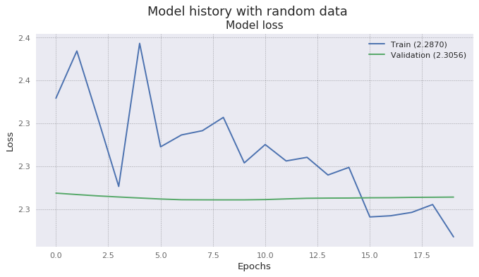
Plot of history
The plot_history function can plot the loss and a metric from the
history.history dictionary usually returned by a Keras model.
Plot of only loss with grid and a different style for matplotlib.
bplt.plot_history(history, title='Model history with random data', grid='both', figsize=(10, 5), style='seaborn')
<matplotlib.axes._subplots.AxesSubplot at 0x7f3f297d78d0>
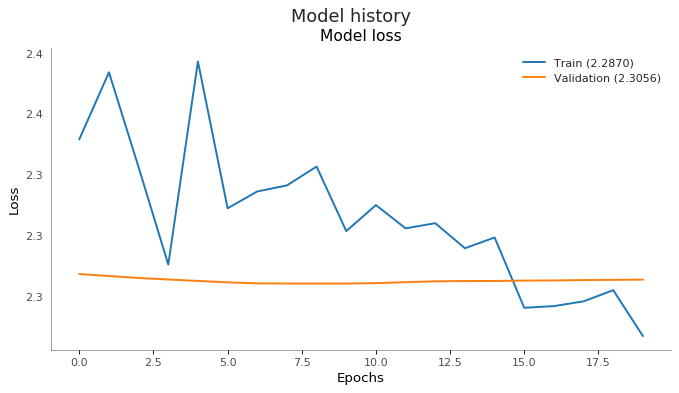
Plot of history using a previously created axis.
__, ax = plt.subplots(1, 1, figsize=(10, 5), dpi=80)
bplt.plot_history(history, axes=ax, style='seaborn')
<matplotlib.axes._subplots.AxesSubplot at 0x7f3f297c34a8>
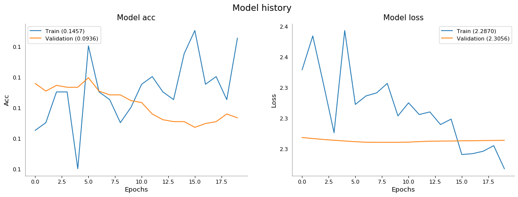
Plot of history with loss and acc.
bplt.plot_history(history, metric='acc')
array([<matplotlib.axes._subplots.AxesSubplot object at 0x7f0fd8b12ac8>,
       <matplotlib.axes._subplots.AxesSubplot object at 0x7f0fd84749b0>],
      dtype=object)
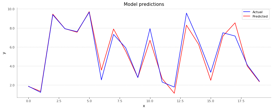
Plot of predictions
Plot of actual and predicted values on the same axis.
bplt.plot_predictions(y_true, y_pred)
<matplotlib.axes._subplots.AxesSubplot at 0x7f0fd8c823c8>
Plot series
Series can either be plot on the same axis or in different ones in the same figure.
Some fake data are created in a DataFrame. The index must be named
datetime. A different color is assigned to each of the acceleration.
AXIS = {'x': 'darkorange', 'y': 'green', 'z': 'steelblue'}
data = (pd.DataFrame(np.random.randint(0, 100, size=(60 * 60, 3)), columns=AXIS.keys())
        .set_index(pd.date_range('2018-01-01', periods=60 * 60, freq='S'))
        .rename_axis('datetime'))

data_miss = (data
             .drop(pd.date_range('2018-01-01 00:05', '2018-01-01 00:07', freq='S'))
             .drop(pd.date_range('2018-01-01 00:40', '2018-01-01 00:41', freq='S'))
             .drop(pd.date_range('2018-01-01 00:57', '2018-01-01 00:59', freq='S'))
             )
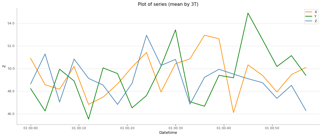
Plot of x, y and z acceleration on the same axis. The function is returning the axis so it can be used in the next plot.
ax = bplt.plot_series(data, 'x', groupby='3T', title=f'Plot of all axis', color=AXIS['x'])
for k in list(AXIS.keys())[1:]:
    bplt.plot_series(data, k, groupby='3T', ax=ax, color=AXIS[k])
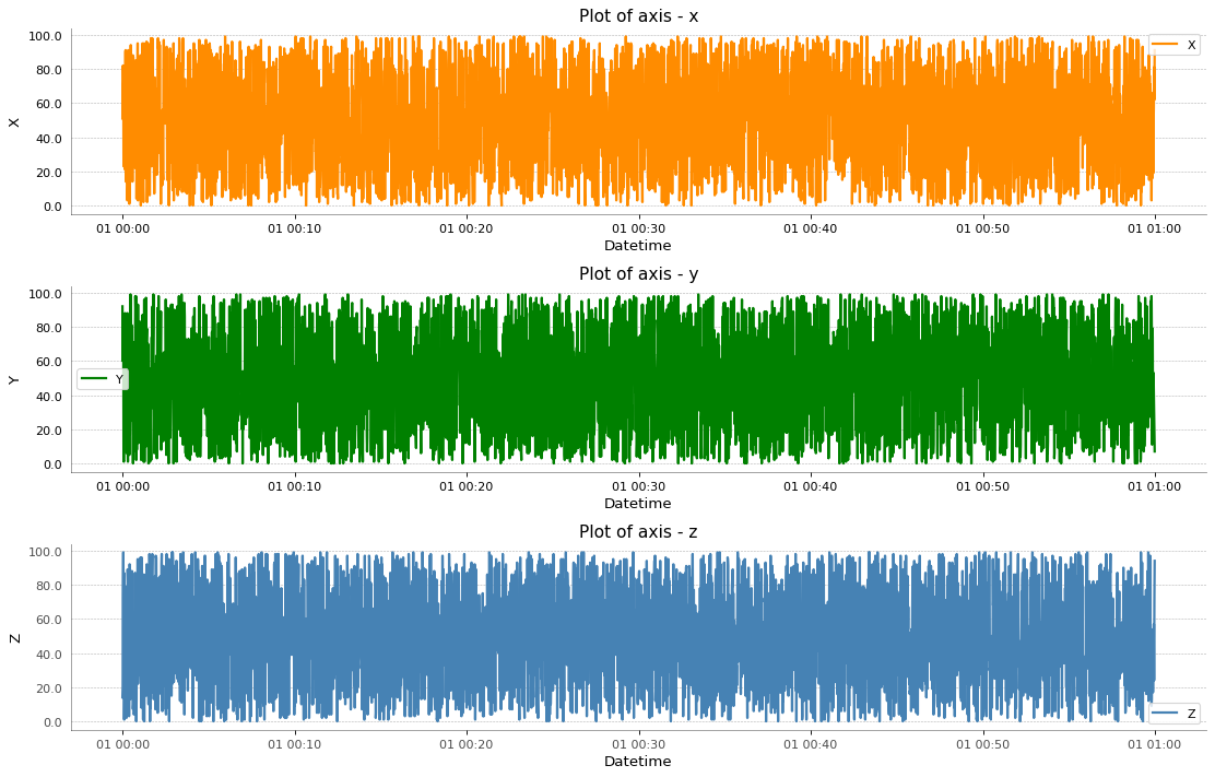
This time, accelerations are plot on a figure containing a different axis for each acceleration.
_, axes = plt.subplots(nrows=len(AXIS), ncols=1, figsize=(14, len(AXIS) * 3), dpi=80)
for i, k in enumerate(AXIS.keys()):
    bplt.plot_series(data, k, ax=axes[i], title=f'Plot of axis - {k}', color=AXIS[k])
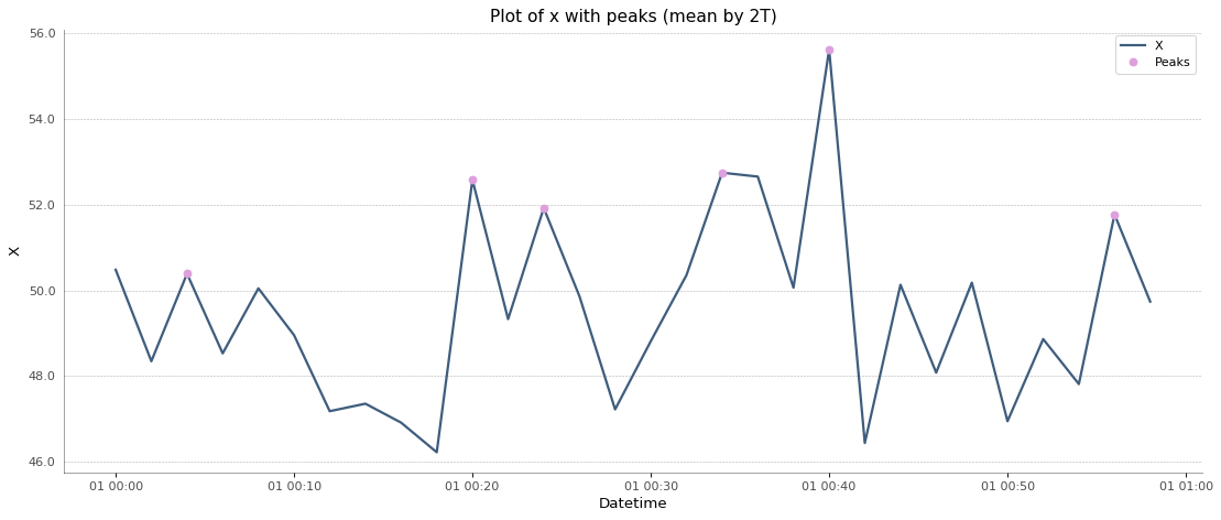
A resampling of the data is done by averaging each 2 minutes (2T). A
peak detection is done as well.
bplt.plot_series(data, 'x', groupby='2T', with_peaks=True, title=f'Plot of x with peaks')
<matplotlib.axes._subplots.AxesSubplot at 0x7f3f2ad91f98>
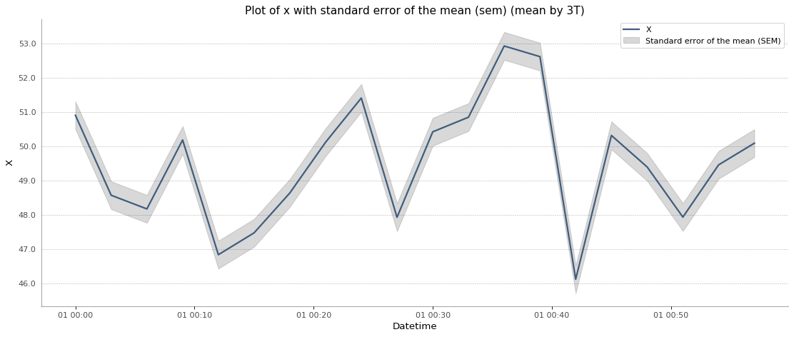
A resampling of the data is done by averaging each 3 minutes (2T).
The standard error of the mean (SEM) is plotted as well. This is usefull
to see if the data are close to the mean or not since there was a
resampling.
bplt.plot_series(data, 'x', groupby='3T', with_sem=True, title=f'Plot of x with standard error of the mean (sem)')
<matplotlib.axes._subplots.AxesSubplot at 0x7f3f29c38668>
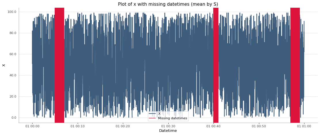
Plot of a serie with missing data. By specifying the resampling, we can easily see if some of the datetime are missing.
bplt.plot_series(data_miss, 'x', groupby='S', with_missing_datetimes=True,
                 title=f'Plot of x with missing datetimes')
<matplotlib.axes._subplots.AxesSubplot at 0x7f3f2a2e58d0>
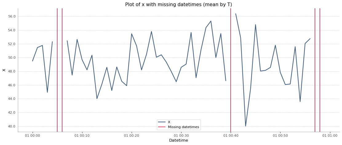
Same as the previous plot, but with a group by minute (T). Since
this is regroup by minute, there are less data missing.
bplt.plot_series(data_miss, 'x', groupby='T', with_missing_datetimes=True,
                 title=f'Plot of x with missing datetimes')
<matplotlib.axes._subplots.AxesSubplot at 0x7f3f2a30c748>
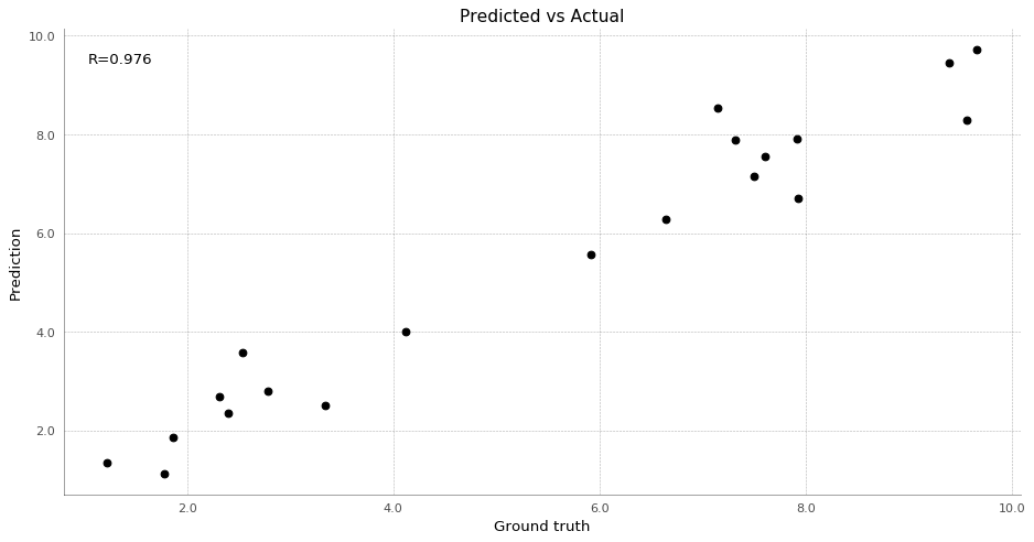
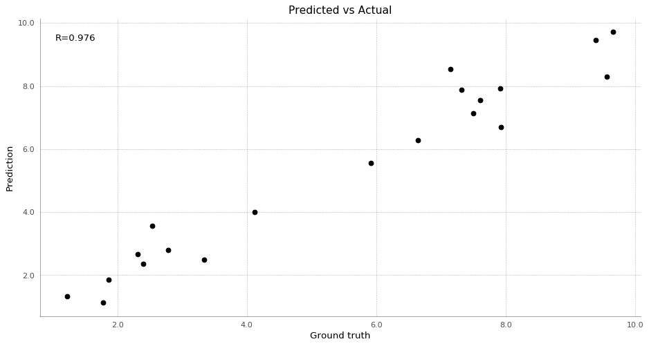
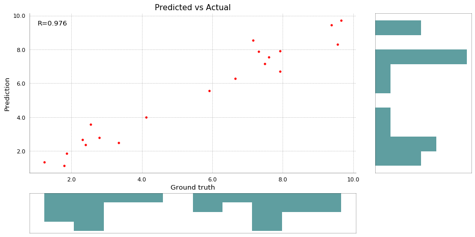
Plot true vs pred
Plot the real data against the predictions. The correlation (R) can
be calculated or not using the with_correlation option.
bplt.plot_true_vs_pred(y_true, y_pred)
<matplotlib.axes._subplots.AxesSubplot at 0x7f0fdae202b0>
Using the with_histograms option, the function will plot histograms
on the side, showing the distribution of the data.
ax = bplt.plot_true_vs_pred(y_true, y_pred, with_histograms=True, marker='.', c='r')
Plot using a previously created axis.
__, ax = plt.subplots(1, 1, figsize=(14, 7), dpi=80)
bplt.plot_true_vs_pred(y_true, y_pred, ax=ax)
<matplotlib.axes._subplots.AxesSubplot at 0x7f3f29b84518>